Numeric Alchemy with Microsoft Excel

Can we turn lead into gold, or even turn budget deficits into budget surpluses using Microsoft Excel? You betcha we can. And the answer lies in rounding – the power to change numbers and blur boundaries in one mighty swoop.

There's nothing cooler than formatting numbers. Select a range and click on the Thousands tool, or the Percentage tool, or click multiple times on the Descending Decimals tool and voila – instant transformation to pretty digits. But there's a fundamental flaw here that can one day end up biting you in the proverbial – and that fundamental flaw is that formatting changes only the presentation of the number, not the number itself.

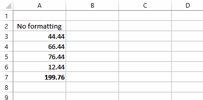
Take these simple numbers for example. Column A shows 4 numbers totalled at the bottom. These are raw, untreated numbers. The 4 numbers add up to 199.76.

When these numbers, including the total, are formatted to zero decimal places you get the result shown here in Column B.

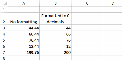
Everything here looks fine but look closely and you'll see that the 4 numbers as shown should add up to 198, not 200 – this is what is referred to as a rounding error. This has occurred because the display of the numbers has changed but the underlying values still used by the summing formula haven't. The sum function in B7 actually adds 44.44 + 66.44 + 76.44 + 12.44. Using formatting the display of each of those values is rounded down. Since the values add up to 199.76 the total is rounded up when formatted to 200.

In the scheme of things this is mostly neither here nor there, unless you're working on something where precision is absolutely critical – you might, for example be counting in billions for the country's economy. Losing or making .24 of a billion might be what keeps you employed!

Rounding errors are eliminated by changing the actual underlying value in the cell. The best way to do this is to use a ROUND() function as shown in the next screen.

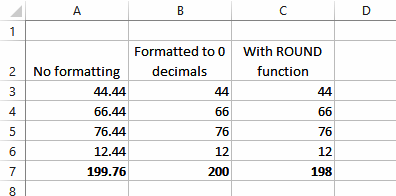
In this example we entered the formula =ROUND(A3,0) into C3. This function has been told to round to zero decimal places. Taking the value 44.44 in A3 the function actually rounds this down to 44. The value of 44, not 44.44, is then the real value in C3. Adding all these four numbers together results in a total of 198.

In a function such as ROUND() the bits required within the brackets are known as parameters. With the ROUND() function we must specify a value to work on (usually a cell reference), and the number of decimals to round to. In our example, this was zero, but it could have been 1, or 2, or whatever.

But the ROUND() function also has an uber-cool operational aspect to it. When you use negative values to specify the decimal places, Excel will start to round to nearest 10s, 100s, 1,000s, or whatever. In this screen we're working with one number and using both formatting and variations of the ROUND() function on it.

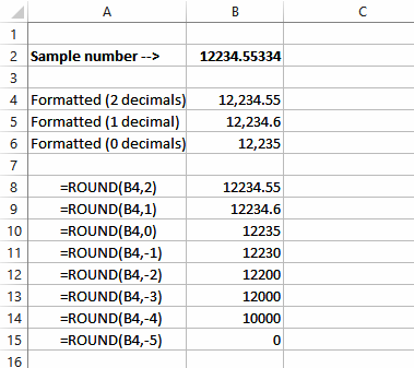
Here we start with 12234.55334 and gradually whittle its presentation down to 12,235 using formatting. A similar result occurs with the first three examples of the ROUND() function, except that we're changing the underlying value.

But magic starts to happen when we using negative values as decimal places. Eventually, by the time we get to -5, we've totally wiped the value out. Mr Treasurer, eat your heart out!

The ROUND() function has spawned 2 offspring over the years: ROUNDUP() rounds numbers up, while ROUNDDOWN() rounds them down. Boy, does life get interesting when these guys are used in the same way.

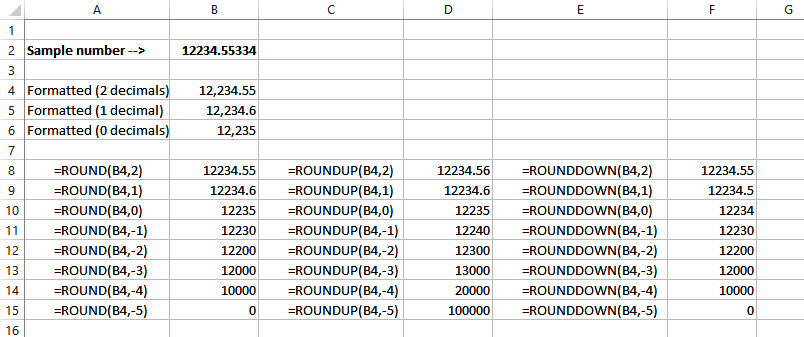
So depending upon whether you use ROUND() or ROUNDUP() or ROUNDDOWN, you can turn 12234.55334 into either 0 or 100,000. Maybe not lead into gold, but certainly numeric alchemy!